Zombie Apocalypse

author: Barron H. Henderson date: 2020-02-11

Inspired by numerous mathematics examples using Zombies (e.g., [1,2,3]), this is a test of the pykpp system to solve for a zombie outbreak.

The basic model is that zombies (Z) both kill and infect humans (H), and humans kill zombies. I have also added a natural death and birth rate for humans, though it makes little difference on the time scales here. I have made additional assumptions as follows:

1. uniform distribution of humans and zombies,

2. interactions are proportional to density,

3. like infectous diseases, the zombie infection rates increase in winter

4. human militarization against zombies increases with the total zombies.

To run this exmaple, you must have installed pykpp

python -m pip install https://github.com/barronh/pykpp/archive/main.zip

[1] https://people.maths.ox.ac.uk/maini/PKM%20publications/384.pdf

[2] https://www.ncbi.nlm.nih.gov/pmc/articles/PMC4798798/

[3] https://www.amazon.com/dp/0691173206/ref=cm_sw_em_r_mt_dp_688KKQ5HMHJW9G6Z6654

import io
import pykpp
import pandas as pd
import numpy as np
import matplotlib.pyplot as plt

Define Reactions

• R1 : Zombies infect humans with a seasonal variation * k_inf is set later as a constant * A multiplier ranging from 0.25 in the summer to 1.75 in the winter

• R2 : zombies kill humans using a constant coefficient

• R3 : humans kill zombies using a coefficient made of two parts: * k_hkillz : humans naturally defend themselves killing zombies * Z * AREA : the military or police gets involved proportional to the total

  zombie population.

  • Right now, human militarization increase with zombie population, but it decreases immediately in response. This is unrealistic. It would be good to add a “memory” so that the zombies are removed more effectively.

• R4, R5 : humans naturally procreate and die

mechanism = """
#EQUATIONS
{R1} Zombie + Human = 2 Zombie + Infected : k_inf * (np.cos(np.radians(t / 365 * 360)) * 0.5 + 1); {infections increase in winter}
{R2} Zombie + Human = Zombie + KilledHuman : k_zkillh;
{R3} Zombie + Human = Human + KilledZombie : k_hkillz * (Zombie * AREA); {humans militarize against zombies proportional to total zombie population}
{R4} Human = 2 Human : k_hbirth;
{R5} Human = DeadHuman : k_hdeath;

"""

Initialize the model

• time (t) is initialized at the start

• the end is set to 10 years hences

• Latitude/Longitude/Temperature/M are unused, but added to satisfy exectations of pykpp

• AREA is set to USA area in km2

• constant rate coefficients are set

• monitoring the Human and Zombie population

• using the scipy.ode integrator

• Finally setting the initial values * CFACTOR is used to convert populations to population/km2 * Humans (H) is set to an approximate USA population * Zombies (Z) is set to a very small initial population

setup = """
#INLINE PY_INIT
t=TSTART=0 # days
TEND=365.25*10+TSTART
TEMP = 288.; # unused
M = 0.; # unused
DT = 3/24.
StartDate = 'datetime(2010, 7, 14)'
Latitude_Degrees = 40. # Unused
Longitude_Degrees = 0.00E+00 # Unused
AREA = 9.834e6 {USA area in km2}
k_inf = 0.5/365 # 0.5 km2/person/year
k_zkillh = 0.2/365 # 0.2 km2/person/year
k_hkillz = 0.1/365 # 0.1 km2/person/year
k_hbirth = 0.01/365 # 1% per year
k_hdeath = 0.01/365 # 1% per year
#ENDINLINE
"""
config = """
#MONITOR Human; Zombie;
#INTEGRATOR odeint;
"""
init = """
#INITVALUES
CFACTOR = 1./AREA {people-to-people/km2 based on USA area}
ALL_SPEC=1e-32*CFACTOR;
Human = 300e6 {approximate US population}
Zombie = 10
"""
mechdef = setup + '\n' + config + '\n' + init + '\n' + mechanism

Load the model

• Using IO to create an in-memory file

• Creating a mechanism: * called ‘zombies’, so the output will be ‘zombies.pykpp.tsv’ * solving at a 1 day increment * monitoring as it is solved per year

mech = pykpp.mech.Mech(
    io.StringIO(mechdef), mechname='zombies', incr=1, monitor_incr=365,
    verbose=0
)

Species: 6
Reactions: 5

Reset and Run

• Run the model and print the total time to solve

runtime = mech.run(verbose=1, debug=False, solver='odeint'); # vode or lsoda
print('Runtime (s)', runtime)

tstart:  0
tend:  3652.5
dt:  0.125
solver_keywords:  {}
{t:0,Human:3E+08,Zombie:10}
odeint {'atol': 0.001, 'rtol': 0.0001, 'mxstep': 1000, 'hmax': 0.125, 'mxords': 2, 'mxordn': 2}
{t:365,Human:3E+08,Zombie:7.3}
{t:730,Human:3E+08,Zombie:7.3}
{t:1095,Human:3E+08,Zombie:7.3}
{t:1460,Human:3E+08,Zombie:7.3}
{t:1826,Human:3E+08,Zombie:7.3}
{t:2191,Human:3E+08,Zombie:7.3}
{t:2556,Human:3E+08,Zombie:7.3}
{t:2921,Human:3E+08,Zombie:7.3}
{t:3286,Human:3E+08,Zombie:7.3}
{t:3651,Human:3E+08,Zombie:7.3}
Runtime (s) 8.203604698181152

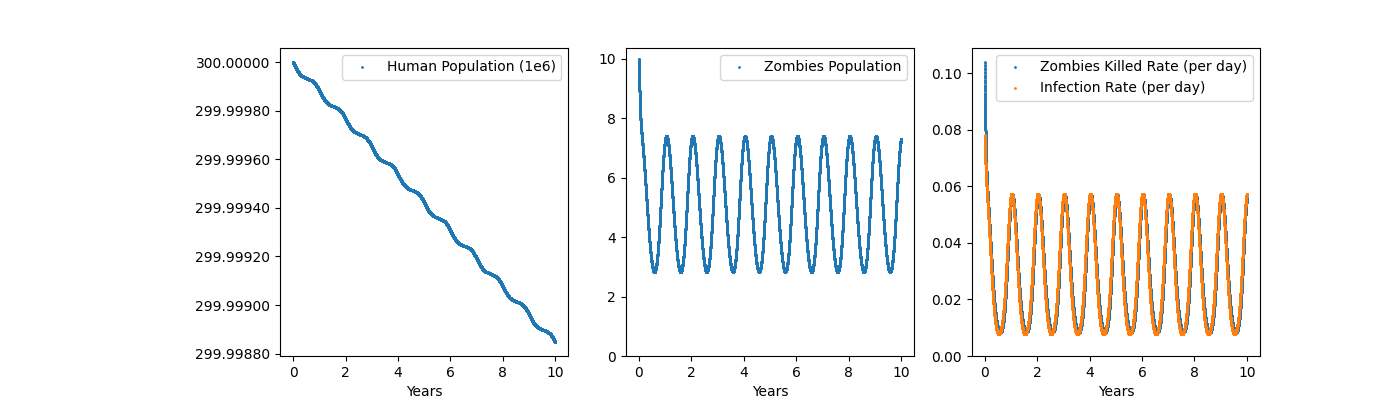
Plot the Zombie Statistics

• Using pandas to read the file

• Using matplotlib for control over plotting.

• note that the seasonality of infection rate causes the wobble.

def zombieplot(tsvpath, timelabel='Years'):
  data = pd.read_csv(tsvpath, delimiter='\t', index_col='t')
  if timelabel.lower() == 'years':
    tfac = 1 / 365.25
  elif timelabel.lower() == 'days':
    tfac = 1
  else:
    raise KeyError(f'timelabel must be Years or Days; got {timelabel}')

  t = data.index.values * tfac
  kH = data.Human / 1e6
  Z = data.Zombie
  dZ = data.KilledZombie
  kI = data.Infected
  gskw = dict(wspace=0.2, left=.2)
  fig, axx = plt.subplots(1, 3, figsize=(14, 4), gridspec_kw=gskw)
  plt.setp(axx, xlabel=timelabel)
  plt.rc('lines', marker='o', linestyle='none', markersize=1)
  axx[0].plot(t, kH, label='Human Population (1e6)')
  mfmt = plt.matplotlib.ticker.FuncFormatter('{0:.5f}'.format)
  axx[0].yaxis.set_major_formatter(mfmt)
  axx[1].plot(t, Z, label='Zombies Population')
  axx[2].plot(t[1:], np.diff(dZ), label='Zombies Killed Rate (per day)')
  axx[2].plot(t[1:], np.diff(kI), label='Infection Rate (per day)')
  for ai, ax in enumerate(axx):
    ax.legend()
  axx[1].set_ylim(0, None);
  axx[2].set_ylim(0, None);
  return fig

fig = zombieplot('zombies.pykpp.tsv')
fig.savefig('zombies.pykpp.png')

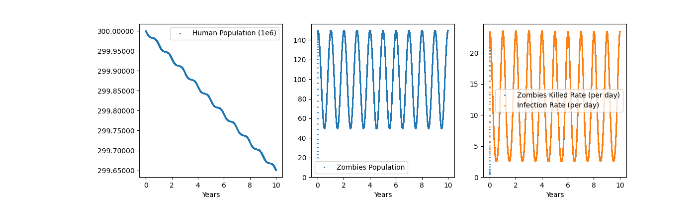
Re run with adjustments parameters

mech = pykpp.mech.Mech(
    io.StringIO(mechdef), mechname='zombies2', incr=1, monitor_incr=365,
    verbose=0
)
# Increase initial Zombies by 2 and the infection rate by 20
mech.world['Zombie'] *= 2
mech.world['k_inf'] *= 20
runtime = mech.run(verbose=1, debug=False, solver='odeint'); # vode or lsoda

fig = zombieplot('zombies2.pykpp.tsv');
fig.savefig('zombies2.pykpp.png')

Species: 6
Reactions: 5
tstart:  0
tend:  3652.5
dt:  0.125
solver_keywords:  {}
{t:0,Human:3E+08,Zombie:20}
odeint {'atol': 0.001, 'rtol': 0.0001, 'mxstep': 1000, 'hmax': 0.125, 'mxords': 2, 'mxordn': 2}
{t:365,Human:3E+08,Zombie:1.5E+02}
{t:730,Human:3E+08,Zombie:1.5E+02}
{t:1095,Human:3E+08,Zombie:1.5E+02}
{t:1460,Human:3E+08,Zombie:1.5E+02}
{t:1826,Human:3E+08,Zombie:1.5E+02}
{t:2191,Human:3E+08,Zombie:1.5E+02}
{t:2556,Human:3E+08,Zombie:1.5E+02}
{t:2921,Human:3E+08,Zombie:1.5E+02}
{t:3286,Human:3E+08,Zombie:1.5E+02}
{t:3651,Human:3E+08,Zombie:1.5E+02}

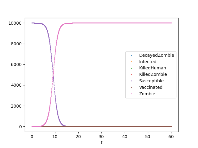
Equations of the End: Teaching Mathematical Modeling Using the Zombie Apocalypse

Lofgren et al. 2016[1] published a teaching example and an on-line playground[2] with solutions. This offers a really cool opportunity to check our results.

We get the exact same results – hooray! Try changing the parameters. For example, adjust the parameters to represent COVID. Consider adding effects of temperature and humidity in transmission.

[1] https://www.ncbi.nlm.nih.gov/pmc/articles/PMC4798798/#s1-jmbe-17-134

[2] http://cartwrig.ht/apps/whitezed/

import pykpp
import pandas as pd
zeddef = """
#EQUATIONS
{R1} Zombie + Susceptible = Zombie + Infected : k_inf;
{R2} Zombie + Susceptible = Zombie + KilledHuman : k_zkillh;
{R3} Zombie + Susceptible = Susceptible + KilledZombie : k_hkillz;
{R5} Zombie = DecayedZombie : k_zdeath;
{R6} Susceptible = Vaccinated : k_vaccination;
{R7} Infected = Zombie : k_incubation;

#INLINE PY_INIT
t=TSTART=0 # days
TEND=TSTART + 60
TEMP = 288.; # unused, but represents average surface temperature
P = 101325.; # unused, but represents average surface pressure
M = P / 8.314 / TEMP * 6.022e23; # unused

DT = 1/24.

StartDate = 'datetime(2010, 7, 14)'
Latitude_Degrees = 40. # Unused
Longitude_Degrees = 0.00E+00 # Unused

k_inf = 1.          {infection rate}
k_zkillh = 0.0      {zombie kill human rate}
k_hkillz = 0.0      {human kill zombie rate}
k_zdeath = 0.0      {zombie decay}
k_vaccination = 0.0 {rate of susceptible vaccination}
incubation_time_days = 1e-3 {must be greater than zero}
k_incubation = 1 / (incubation_time_days) { tau = 1 / k; so tau = 1 seconds}
#ENDINLINE

#MONITOR Susceptible; Vaccinated; Zombie;
#INTEGRATOR odeint;

#INITVALUES
CFACTOR = 1./10001 { denominator should match sum of people = Susceptible + Vaccinated + Zombie}
ALL_SPEC=1e-32*CFACTOR;
Susceptible = 10000
Vaccinated = 0
Zombie = 1
"""
mech = pykpp.mech.Mech(
    io.StringIO(zeddef), mechname='zed', incr=1/24, monitor_incr=5, verbose=0
)
runtime = mech.run(verbose=1, debug=False, solver='odeint'); # vode or lsoda

data = pd.read_csv('zed.pykpp.tsv', delimiter='\t', index_col='t')
ax = data.drop(['TEMP', 'P', 'CFACTOR'], axis=1).plot()
ax.figure.savefig('zed.pykpp.png')

Species: 7
Reactions: 6
tstart:  0
tend:  60
dt:  0.041666666666666664
solver_keywords:  {}
{t:0,Susceptible:1E+04,Vaccinated:0,Zombie:1}
odeint {'atol': 0.001, 'rtol': 0.0001, 'mxstep': 1000, 'hmax': 0.041666666666666664, 'mxords': 2, 'mxordn': 2}
{t:5,Susceptible:9.9E+03,Vaccinated:0,Zombie:1.5E+02}
{t:10,Susceptible:3.1E+03,Vaccinated:0,Zombie:6.9E+03}
{t:15,Susceptible:30,Vaccinated:0,Zombie:1E+04}
{t:20,Susceptible:0.22,Vaccinated:0,Zombie:1E+04}
{t:25,Susceptible:0.0016,Vaccinated:0,Zombie:1E+04}
{t:30,Susceptible:1.1E-05,Vaccinated:0,Zombie:1E+04}
{t:35,Susceptible:8.3E-08,Vaccinated:0,Zombie:1E+04}
{t:40,Susceptible:5.8E-10,Vaccinated:0,Zombie:1E+04}
{t:45,Susceptible:4E-12,Vaccinated:0,Zombie:1E+04}
{t:50,Susceptible:2.9E-14,Vaccinated:0,Zombie:1E+04}
{t:55,Susceptible:2E-16,Vaccinated:0,Zombie:1E+04}