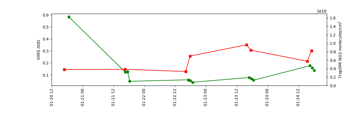
NYC VIIRS AOD vs TropOMI NO2

Timeseries comparison of VIIRS AOD and TropOMI in NYC.

import matplotlib.pyplot as plt
import pyrsig
import os

os.makedirs('nyc', exist_ok=True)

# Create an RSIG api isntance
# Define a Time and Space Scope: here end of February around Phoenix
rsigapi = pyrsig.RsigApi(
    bdate='2022-01-20', edate='2022-01-25',
    bbox=(-74.8, 40.32, -71.43, 41.4), workdir='nyc'
)

# Get TropOMI NO2
tomino2df = rsigapi.to_dataframe(
    'tropomi.offl.no2.nitrogendioxide_tropospheric_column',
    unit_keys=False, parse_dates=True
)

# Get VIIRS AOD
viirsaoddf = rsigapi.to_dataframe(
    'viirsnoaa.jrraod.AOD550', unit_keys=False, parse_dates=True
)

# Create spatial medians for TropOMI and AQS
tomids = (
    tomino2df.groupby('time').median(numeric_only=True)['nitrogendioxide_tropospheric_column']
)
viirsds = (
    viirsaoddf.groupby('time').median(numeric_only=True)['AOD550']
)

# Create axes with shared x
fig, ax = plt.subplots(figsize=(12, 4),
                       gridspec_kw=dict(bottom=0.25, left=0.15, right=0.95))
ax.tick_params(axis='x', labelrotation = 90)
tax = ax.twinx()

# Add VIIRS AOD
ax.plot(viirsds.index.values, viirsds.values, marker='o', color='g')

# Add TropOMI NO2
tax.plot(tomids.index.values, tomids.values, marker='s', color='r')

# Configure axes
ax.set(ylabel='VIIRS AOD')
tax.set(ylim=(0, 1.7e16), ylabel='TropOMI NO2 molecules/cm$^2$')

plt.show()
# Or save out figure
# fig.savefig('nyc.png')