Domain-wide Gridded Emission Scaling

Apply a constant factor to a subset of emission variables in a file.

The basic steps are:

1. Copy a file.

2. Select species to scale NOx species.

3. Scale by a multiplicative factor.

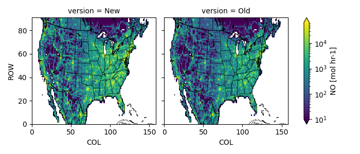
4. Plot the old and new result.

Reminder: You must have already activated your python environment.

Configuration

# date to process
date = '20160610'
# file to copy
oldpath = f'../../camx/emiss/camx_area.mobile.{date}.36km.nc'
# new file to create
newpath = f'outputs/camx_area_2x.mobile.{date}.36km.nc'
# species to scale
scalekeys = ['NO', 'NO2', 'HONO']  # list of strings or set to 'all'
# factor to scale by
factor = 2.
# path for figure comparing
figpath = 'outputs/scaled_gridemiss_scalewholedomain.png'

Imports and File Prep

import netCDF4
import shutil
import os

os.makedirs('outputs', exist_ok=True)
shutil.copyfile(oldpath, newpath)

'outputs/camx_area_2x.mobile.20160610.36km.nc'

Open Files

• Open the existing file in read-only mode

• Open the new file in editable append mode

infile = netCDF4.Dataset(oldpath, mode='r')
outfile = netCDF4.Dataset(newpath, mode='a')

Select Emission Variables to Scale

• if scalekeys is all, identify all emission variables by unit

if scalekeys == 'all':
    scalekeys = [
        k for k, v in outfile.variables.items()
        if v.units.strip() in ('mol hr-1', 'g hr-1')
    ]

noscalekeys = sorted(set(outfile.variables).difference(scalekeys))
print('INFO:: no scale', noscalekeys)
print('INFO:: to scale', scalekeys)

INFO:: no scale ['ACET', 'ALD2', 'ALDX', 'BENZ', 'BNZA', 'CH4', 'CO', 'CPRM', 'ECH4', 'ETFLAG', 'ETH', 'ETHA', 'ETHY', 'ETOH', 'FORM', 'FPRM', 'IOLE', 'ISOP', 'ISP', 'IVOA', 'KET', 'MEOH', 'NA', 'NH3', 'NVOL', 'OLE', 'PAL', 'PAR', 'PCA', 'PCL', 'PEC', 'PFE', 'PH2O', 'PK', 'PMG', 'PMN', 'PNH4', 'PNO3', 'POA', 'PRPA', 'PSI', 'PSO4', 'PTI', 'SO2', 'SULF', 'TERP', 'TFLAG', 'TOL', 'TOLA', 'TRP', 'UNK', 'UNR', 'X', 'XYL', 'Y', 'latitude', 'longitude']
INFO:: to scale ['NO', 'NO2', 'HONO']

Apply Scaling

for skey in scalekeys:
    print('INFO:: scaling', skey, 'by', factor)
    outvar = outfile.variables[skey]
    invar = infile[skey]
    outvar[:] = factor * invar[:]

outfile.sync()
del outfile

INFO:: scaling NO by 2.0
INFO:: scaling NO2 by 2.0
INFO:: scaling HONO by 2.0

Plot Comparison

import pyrsig
import pycno
import matplotlib.colors as mc

oldfile = pyrsig.open_ioapi(oldpath)
newfile = pyrsig.open_ioapi(newpath)
key = scalekeys[0]
compfile = newfile[[]]
compfile['New'] = newfile[key].sum('LAY').mean('TSTEP')
compfile['Old'] = oldfile[key].sum('LAY').mean('TSTEP')
Z = compfile.to_dataarray(dim='version')
Z.attrs.update(oldfile[key].attrs)
fca = Z.plot(col='version', norm=mc.LogNorm(10, compfile['Old'].max()))
pycno.cno(oldfile.crs_proj4).drawstates(ax=fca.axs)
fca.fig.savefig(figpath)