Examples¶

Get System Ready¶

The first step to running examples is to prepare the computer on. The examples can be run on Linux, Mac (OS X), or Windows machines. Some of the instructions will assume you are in a terminal (Linux or Mac), but can be adapted to Windows Command Prompt or PowerShell.

Steps:

Download examples folder.
Setup a python version
- Either with a system Python
- Or mamba.
Get CAMx tutorial files.

Once you have done all these steps, you should will be ready to run example scripts. The scripts use file paths to “point” to files assuming a relative folder structure. Each python script (eg, run_gridemiss_01_perturb.py) will be run using python from within its folder (eg, examples/gridemiss/). So, it is important that the folder structure is as expected or you edit the paths in the scripts.

So, if you were done preparing the system (steps 1-3), you would run an example script like this on Linux or Mac:

cd ~
cd examples/gridemiss
python run_gridemiss_01_perturb.py

Or Windows PowerShell

cd ~
cd examples/gridemiss
py.exe run_gridemiss_01_perturb.py

As an alternative, you can run these script by pasting sections of them into an interactive Python console. For example, on Linux/Mac:

cd ~/examples/gridemiss
python
>>> # paste commands here

Or in Windows PowerShell:

cd ~/examples/gridemiss
py.exe
>>> # paste commands here

Remember, this will not work until you complete the preparation steps:

Getting the examples folder done in Get Examples Folder
Preparing the python executable is described in the Preparing Python Environment (or in the Using Mamba to get Python).
Getting the CAMx tutorial data is described in the Getting CAMx Files example.

Get Examples Folder

Preparing Python Environment

Using Mamba to get Python

Getting CAMx Files

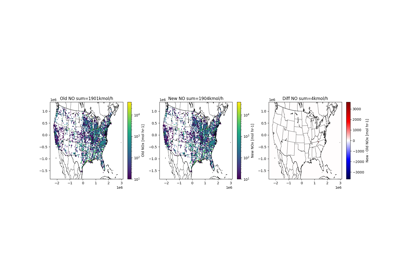
Gridded Emission Examples¶

There are currently two gridded emission examples:

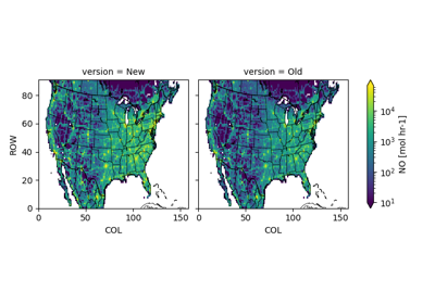
Scale gridded emissions across the whole domain.
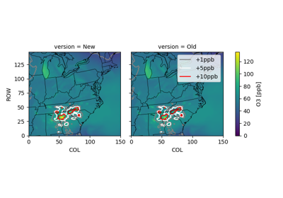
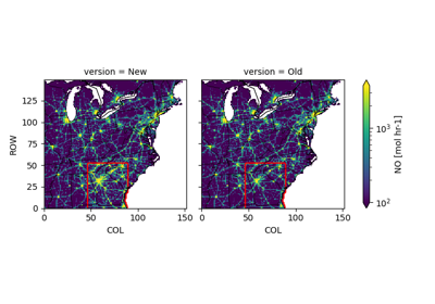
Scale gridded emissions in a specific region.

Caveat: The “specific region” can be modified to be very specific, but has limits. The examples work from emissions that have already been gridded, speciated, and often merged across many “sectors.” When trying to make very specific updates (e.g, a single SCC), sometimes this approach will fall short.

Domain-wide Gridded Emission Scaling

Region-specific Gridded Emission Scaling

Point Source Emission Examples¶

There are currently two point source examples:

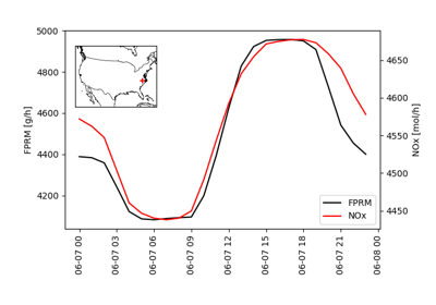
Make a single representative source file.
Perturb a facilities based on latitude/longitude.

Caveat: These point source examples can be adapted to do many things, but there are limitations. For example, sometimes “point source emissions” are split between the amount subject to plume rise and the rest may be merged with the gridded. In that case, scaling the point source file is not equivalent to scaling a facility.

Create a Hypothetical Source

Modify a Selected Source

Rerun CAMx¶

Edit run script to use edited emission files.
Run CAMx as you normally would.

Rerun CAMx with Updated Emissions

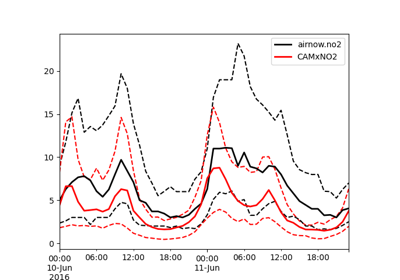
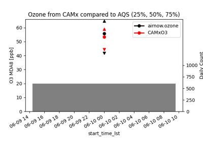
Model Performance Evaluation¶

There are currently two model performance examples. These are meant to be instructive and do not cover all possibilities. These examples use EPA’s RSIG to aquire AirNow or AQS observations, which is useful for rapid evaluation and retrospective evalaution.

Compare CAMx to hourly NO2.
Compare CAMx to Ozone Maximum Daily 8-hour Average.

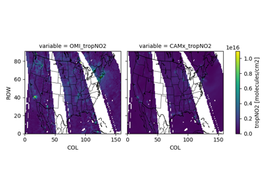
Compare Model to Hourly Observations

Compare Model to Daily MDA8 Observations

Satellite Comparison¶

There are currently two satellite processing examples.

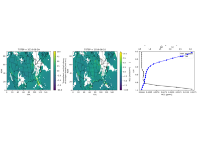
OMI NO2 comparison without updating the model prior, and
TropOMI NO2 comparison with an updated model prior.

Satellite NO2 use modeled NO2 (eg, GMI or TM5) to quantify the vertical distribution of NO2, which allows for a quantitative translation from measurements with differential vertical sensitivity to a best estimate assuming equal sensitivity. Using your own model as the vertical distribution ensures an apples to apples comparison.