Simple OMI

This example compares CAMx to the Ozone Monitoring Instrument (OMI) for NO2 tropospheric vertical column densitities (tropNO2). OMI’s tropNO2 is derived from a measurement along the path light from the sun and reflected off the surface of the earth. The original measurement is called a slant column density (SCD). The SCD is split into tropospheric and stratospheric parts, based on a model profile (a priori). The a priori and slant path are combined with a sensitivity vector (scattering weight) to convert the tropospheric SCD to tropNO2 [molecules/cm2]. CAMx can output mixing ratios at all levels, which can be converted to molecules/cm2 and summed to make a tropNO2 product. Note, however, that the CAMx tropNO2 inherently assumes a different model profile. A more complete comparison would adjust OMI to use CAMx’s profile, or adjust CAMx to use OMI’s profile. Each has strengths and weaknesses.

Reminder: You must have already activated your python environment.

Imports and Folders

import pyrsig
import os

os.makedirs('outputs', exist_ok=True)

Configuration

cdate = '20160610'    # Using first available CAMx date
odate = '2017-06-10'  # oddly Jun 10-11 of 2016 have no OMI over the US

# Use dates to find avrg file and 3d met file
cpath = f'../../camx/outputs/CAMx.v7.32.36.12.{cdate}.3D.avrg.grd01.nc'
# If you used camx.tar.gz for inputs, update the met folder to metss
mpath = f'../../camx/met/camx.3d.36km.{cdate}.nc'

# Define output paths.
outstem = f'outputs/OMINO2_CAMx.v7.32.36.12.{cdate}.3D.avrg.grd01'
outpath = outstem + '.nc'
tilepath = outstem + '_tile.png'
scatterpath = outstem + '_scatter.png'

Data Acquisition

# Open a CAMx 3D CONC file for NO2
cf = pyrsig.open_ioapi(cpath)
# Open a 3d met file (pressure, z, temperature, humiditiy) and match avrg file time
mkeys = ['pressure', 'z', 'temperature', 'humidity']
mf = pyrsig.open_ioapi(mpath)[mkeys].interp(TSTEP=cf.TSTEP)

# Process OMI for the CAMx grid
api = pyrsig.RsigApi(bbox=(-130, 20, -60, 60), workdir='outputs', grid_kw=cf.attrs)
omids = api.to_ioapi('omi.l2.omno2.ColumnAmountNO2Trop', bdate=odate)

Derive Conversion Factors

• OMI tropospheric NO2 column (tropNO2) in molecules/cm2

• CAMx average mixing ratios (X) in ppmV of dry-air by layer (k)

• Need dry-air intensity (I) molecules/cm2 by layer

• CAMx tropNO2 = $sum_k{X(k) * I(k)}$

# Calculate layer depths from interface heights
dz = mf['z'].copy()
dz[:, 1:] = mf['z'].diff('LAY').data

# Combine pressure, temperature, humidity, and dz to get dry-air intensity
molecules_per_cm2 = (
    mf['pressure'] * 100          # mb -> Pa
    / 8.314 / mf['temperature']   # Pa -> moles/m3
    * (1 - mf['humidity'] / 1e6)  # moles/m3 -> moles_dry/m3
    * dz * 6.022e23 / 1e4         # moles_dry/m3 -> molecules_dry/m2
)
vcdno2 = (cf['NO2'] * 1e-6 * molecules_per_cm2.data).sum('LAY', keepdims=True)
vcdno2.attrs.update(
    long_name='CAMx_tropNO2', units='molecules/cm2',
    var_desc='Simple sum of molecules'
)

Organizing for output

# Allowing OMI coordinates (time) to override CAMx.
omids['CAMx_tropNO2'] = vcdno2.dims, vcdno2.data, vcdno2.attrs

# Mask missing values from OMI.
outf = omids.where(omids['COLUMNAMOUNTNO2'] > -9e36)
# Make OMI naming more clear.
outf = outf.rename(COLUMNAMOUNTNO2='OMI_tropNO2')
outf['OMI_tropNO2'].attrs.update(long_name='OMI_tropNO2')
# Save to disk
pyrsig.cmaq.save_ioapi(outf.drop_vars('TFLAG'), outpath)

Visualize Results

import matplotlib.pyplot as plt
import matplotlib.colors as mc
import pyrsig
import pycno
import numpy as np
from scipy.stats import linregress

# Average potential overlapping overpasses
omids = pyrsig.open_ioapi(outpath).mean(('TSTEP', 'LAY'))

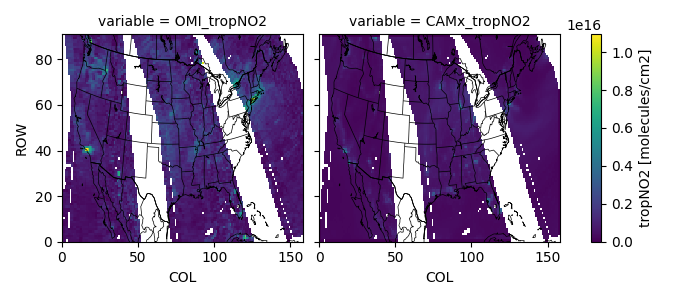
Make a tile-plot

Z = omids[['OMI_tropNO2', 'CAMx_tropNO2']].to_dataarray()
Z.attrs.update(long_name='tropNO2', units='molecules/cm2')
fca = Z.plot(col='variable')
pycno.cno(omids.crs_proj4).drawstates(ax=fca.axs)
fca.fig.savefig(tilepath)

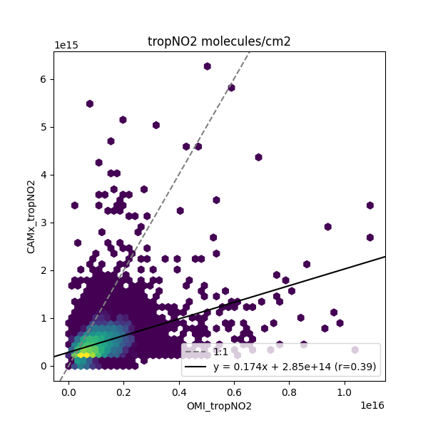
Make a scatter-plot

# Get values from OMI and CAMx separately
omivals = omids['OMI_tropNO2'].to_numpy().ravel()
camxvals = omids['CAMx_tropNO2'].to_numpy().ravel()
bothvalid = ~(np.isnan(omivals) | np.isnan(camxvals))

# Perform least-square regression
lr = linregress(omivals[bothvalid], camxvals[bothvalid])
lrlabel = f'y = {lr.slope:.3}x + {lr.intercept:.3} (r={lr.rvalue:.2f})'

# Create a hexbin plot
fig, ax = plt.subplots(figsize=(6, 6))
pc = ax.hexbin(x=omivals[bothvalid], y=camxvals[bothvalid], gridsize=50, norm=mc.LogNorm(20))
ax.set(xlabel='OMI_tropNO2', ylabel='CAMx_tropNO2', title='tropNO2 molecules/cm2')
ax.axline((0, 0), slope=1, label='1:1', color='grey', linestyle='--')
ax.axline((0, lr.intercept), slope=lr.slope, label=lrlabel, color='k')
ax.legend()
fig.savefig(scatterpath)