Create a Hypothetical Source

This example averages all other sources to create a single hypothetical source. It also reports all variables that are in the file, which makes direct modification easy.

The basic steps are:

1. Read in an existing point source file.

2. Average all points (points are COL dimension).

3. Save out result.

4. Visualize result.

Reminder: You must have already activated your python environment.

Configuration

# what date are you processing?
date = '20160610'
# existing point source file to copy
oldpath = f'../../camx/ptsrce/point.camx.ptnonipm.{date}.nc'
# new point source file for 1 "average" source
newpath = f'outputs/point.camx.just1.{date}.nc'
# plot that demonstrates new file
figpath = 'outputs/example_ptsrce_newsinglesource.png'

Imports

import PseudoNetCDF as pnc
import os

Pepare Folders

os.makedirs('outputs', exist_ok=True)
if os.path.exists(newpath):
    os.remove(newpath)

Create an Average Single Source File

• Old file has N point sources.

• Oddly, each point source is an element of the COL dimension.

oldfile = pnc.pncopen(oldpath)

# Create a Single Source File At Maximum Emission
# '''''''''''''''''''''''''''''''''''''''''''''''
# - Old file has N point sources.
# - Find the stack whose daily average rate is the highest

# Or, create a file based on the maximum stack NO rate
dayfile = oldfile.apply(TSTEP='mean')         # get the mean daily-rate
idx = dayfile.variables['NO'][0, :].argmax()  # find the maximum stack index
atmaxfile = oldfile.slice(COL=idx)              # choose that stack to represent
atmaxfile


# Optional Adjustments
# ''''''''''''''''''''
# There are an infinite number of adjustments you could apply. The examples
# cover relocating the source, modifying the temporal profile and adjusting
# the magnitude.
#
# - Apply the mean temporal profile to the max stack.
# - Relocate the stack to any location.
# - Scale NO by 2

# Calculate the average time profile by species
# note: time profiles are in UTC and averaged across timezones
meanfile = oldfile.apply(COL='mean')
timeprofile = meanfile / meanfile.apply(TSTEP='mean')

# apply the time profiles to the maximum stack's daily average
newfile = atmaxfile.apply(TSTEP='mean') * timeprofile

# Make sure that math did not affect TFLAG
newfile.variables['TFLAG'][:] = atmaxfile.variables['TFLAG'][:]
newfile.variables['ETFLAG'][:] = atmaxfile.variables['ETFLAG'][:]

# Optionally, relocate the hypothetical stack
lon, lat = -78.6382, 35.7796  # Arbitrarily chose Raleigh, NC
proj = newfile.getproj(withgrid=False, fromorigin=True)  # get a pyproj object
x, y = proj(lon, lat)  # calculate the x/y location in meters from LCC center
newfile.variables['xcoord'][:] = x  # assign results
newfile.variables['ycoord'][:] = y

# Optionally, scale a specific set of species
newfile.variables['NO'][:] *= 0.5
newfile.variables['NO2'][:] *= 0.5
newfile.variables['HONO'][:] *= 0.5

# Save the single stack file
# ''''''''''''''''''''''''''

saved = newfile.save(newpath, format='NETCDF4_CLASSIC', outmode='ws')
saved.close()

<string>:1: RuntimeWarning: invalid value encountered in divide
**PNC:/work/ROMO/users/bhenders/SESARMTraining/py312/lib64/python3.12/site-packages/PseudoNetCDF/pncwarn.py:24:UserWarning:
  Currently not using:false_northing 1872000.0
**PNC:/work/ROMO/users/bhenders/SESARMTraining/py312/lib64/python3.12/site-packages/PseudoNetCDF/pncwarn.py:24:UserWarning:
  Currently not using:false_easting 2556000.0
Adding dimensions
Adding globals
Adding variables
Defining xcoord
Defining ycoord
Defining stkheight
Defining stkdiam
Defining stktemp
Defining stkspeed
Defining pigflag
Defining saoverride
Defining TFLAG
Defining ETFLAG
Defining flowrate
Defining plumerise
Defining plume_bottom
Defining plume_top
Defining NO
Defining NO2
Defining OLE
Defining PAR
Defining TOL
Defining XYL
Defining FORM
Defining ALD2
Defining ETH
Defining CO
Defining HONO
Defining ISOP
Defining MEOH
Defining ETOH
Defining SO2
Defining SULF
Defining ALDX
Defining ETHA
Defining IOLE
Defining TERP
Defining NH3
Defining HCL
Defining CL2
Defining CH4
Defining TOLA
Defining ISP
Defining TRP
Defining PSO4
Defining PNO3
Defining POA
Defining PEC
Defining PFE
Defining PMN
Defining PK
Defining PCA
Defining PMG
Defining PAL
Defining PSI
Defining PTI
Defining FPRM
Defining CPRM
Defining PRPA
Defining BENZ
Defining ETHY
Defining ACET
Defining KET
Defining ECH4
Defining UNR
Defining NVOL
Defining PNH4
Defining PCL
Defining PH2O
Defining NA
Defining BNZA
Defining IVOA
Populating xcoord
Populating ycoord
Populating stkheight
Populating stkdiam
Populating stktemp
Populating stkspeed
Populating pigflag
Populating saoverride
Populating TFLAG
Populating ETFLAG
Populating flowrate
Populating plumerise
Populating plume_bottom
Populating plume_top
Populating NO
Populating NO2
Populating OLE
Populating PAR
Populating TOL
Populating XYL
Populating FORM
Populating ALD2
Populating ETH
Populating CO
Populating HONO
Populating ISOP
Populating MEOH
Populating ETOH
Populating SO2
Populating SULF
Populating ALDX
Populating ETHA
Populating IOLE
Populating TERP
Populating NH3
Populating HCL
Populating CL2
Populating CH4
Populating TOLA
Populating ISP
Populating TRP
Populating PSO4
Populating PNO3
Populating POA
Populating PEC
Populating PFE
Populating PMN
Populating PK
Populating PCA
Populating PMG
Populating PAL
Populating PSI
Populating PTI
Populating FPRM
Populating CPRM
Populating PRPA
Populating BENZ
Populating ETHY
Populating ACET
Populating KET
Populating ECH4
Populating UNR
Populating NVOL
Populating PNH4
Populating PCL
Populating PH2O
Populating NA
Populating BNZA
Populating IVOA

Visualize Source to confirm operational

import PseudoNetCDF as pnc
import matplotlib.pyplot as plt
import pycno

# open file and get coordinate information
newfile = pnc.pncopen(newpath, format='netcdf')
proj = newfile.getproj(projformat='proj4', withgrid=False, fromorigin=True)
t = newfile.getTimes()
x = newfile.variables['xcoord'][:]
y = newfile.variables['ycoord'][:]

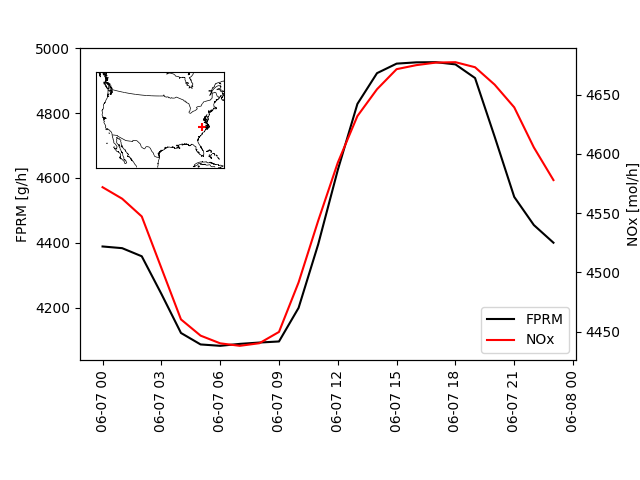
# Create a plot with a primary axis for FPRM, a secondary axis for NOx,
# and an inset axis for spatial location.
gskw = dict(bottom=0.25, top=.9)
fig, ax = plt.subplots(gridspec_kw=gskw)
sax = ax.twinx()
mapax = fig.add_axes([.15, .65, .2, .2])

# Add outlines of countries to the map.
cno = pycno.cno(proj=proj, xlim=(-2.5e6, 2.5e6), ylim=(-2e6, 2e6))
cno.drawcountries(ax=mapax)
# add a point for the source
mapax.scatter(x=x, y=y, marker='+', color='r')
mapax.set(xticks=[], yticks=[])

# Add a time-series plot of FPRM to the primary axis
ax.plot(t, newfile.variables['FPRM'][:, 0], label='FPRM', color='k')
ax.set(ylabel='FPRM [g/h]')
# Add a time-series plot of NOx to the secondary axis
noxf = newfile.eval('NOx = NO[:] + NO2[:] + HONO[:]')
sax.plot(t, noxf.variables['NOx'][:, 0], label='NOx', color='r')
sax.set(ylabel='NOx [mol/h]')

# Orient the date tick labels
plt.setp(ax.get_xticklabels(), rotation=90)
# Add a legend for both axes
ll = ax.lines + sax.lines
ax.legend(ll, [_l.get_label() for _l in ll], loc='lower right')
# Save the figure to disk
fig.savefig(figpath)

**PNC:/work/ROMO/users/bhenders/SESARMTraining/py312/lib64/python3.12/site-packages/PseudoNetCDF/pncwarn.py:24:UserWarning:
  Currently not using:false_northing 1872000.0
**PNC:/work/ROMO/users/bhenders/SESARMTraining/py312/lib64/python3.12/site-packages/PseudoNetCDF/pncwarn.py:24:UserWarning:
  Currently not using:false_easting 2556000.0

Extra Credit

1. Modify the script to set the xcoord and yxoord to a new location before saving out [LCC meters].

2. What other properties might you want to change?