Modify a Selected Source

Point sources may be facilities or individual stacks. This example demonstrates how to apply a scaling factor to all sources in some region. The region can be as simple as a rectangular box, a circle, or any geographic shape you can define.

The basic steps are:

1. Copy an existing emissions file.

2. Define an area within which to apply emissions sclaing.

3. Define a multiplicative scaling factor

4. Apply the scaling factor to all cells within the area.

5. Make a plot demonstrating the change.

Reminder: You must have already activated your python environment.

Configuration

Find a source in the in “Online 2020 NEI Data Retrieval Tool” https://www.epa.gov/air-emissions-inventories/2020-national-emissions-inventory-nei-data - As an example, I chose single stack with the largest NO rate; then updated

the lon/lat to the nearest source in the NEI 2020 inventory

• You’ll have a chance to adjust your shape until you capture the intended source.

# date to process
date = '20160610'
# file to copy
oldpath = f'../../camx/ptsrce/point.camx.ptnonipm.{date}.nc'
# new file to create
newpath = f'outputs/point.camx.ptnonipm_edit.{date}.nc'
# figure demonstrating change
figpath = 'outputs/example_ptsrce_scaleregion.png'

# Region to modify
shape = 'box'  # box, circle, or custom
center = (-82.5436, 36.5224)
dx = 250  # m (used as radius for circle)
dy = 250  # m (ignored for circle)


# factor to apply within the shape
scalekeys = ['NO', 'NO2', 'HONO']  # a list of species or 'all'
factor = 1.2

Imports and Folders

import numpy as np
import netCDF4
import pyproj
import shutil
from shapely import points, box
import os

Define Output and Remove if it exists

• Use an existing file as a template

• Create a copy for direct modification

os.makedirs('outputs', exist_ok=True)
if os.path.exists(newpath):
    os.remove(newpath)

shutil.copyfile(oldpath, newpath)

'outputs/point.camx.ptnonipm_edit.20160610.nc'

Open Files

• Open the existing file in read-only mode

• Open the new file in append mode

oldf = netCDF4.Dataset(oldpath, mode='r')
newf = netCDF4.Dataset(newpath, mode='a')

Select Emission Variables to Scale

If scalekeys is all, select all emission variables by units

if scalekeys == 'all':
    scalekeys = [
        k for k, v in newf.variables.items()
        if v.units.strip() in ('mol hr-1', 'g hr-1')
    ]

noscalekeys = sorted(set(newf.variables).difference(scalekeys))
print('INFO:: no scale', noscalekeys)
print('INFO:: to scale', scalekeys)

INFO:: no scale ['ACET', 'ALD2', 'ALDX', 'BENZ', 'BNZA', 'CH4', 'CL2', 'CO', 'CPRM', 'ECH4', 'ETFLAG', 'ETH', 'ETHA', 'ETHY', 'ETOH', 'FORM', 'FPRM', 'HCL', 'IOLE', 'ISOP', 'ISP', 'IVOA', 'KET', 'MEOH', 'NA', 'NH3', 'NVOL', 'OLE', 'PAL', 'PAR', 'PCA', 'PCL', 'PEC', 'PFE', 'PH2O', 'PK', 'PMG', 'PMN', 'PNH4', 'PNO3', 'POA', 'PRPA', 'PSI', 'PSO4', 'PTI', 'SO2', 'SULF', 'TERP', 'TFLAG', 'TOL', 'TOLA', 'TRP', 'UNR', 'XYL', 'flowrate', 'pigflag', 'plume_bottom', 'plume_top', 'plumerise', 'saoverride', 'stkdiam', 'stkheight', 'stkspeed', 'stktemp', 'xcoord', 'ycoord']
INFO:: to scale ['NO', 'NO2', 'HONO']

Define relevant sources

• Create a projection

• Define an area to scale in

  • in a rectangle,

  • in a circle, or

  • within a complex custom shape

attrs = {k: oldf.getncattr(k) for k in oldf.ncattrs()}
proj4tmpl = '+proj=lcc +lat_0={YCENT} +lon_0={P_GAM}'
proj4tmpl += ' +lat_1={P_ALP} +lat_2={P_BET} +R=6370000 +units=m +no_defs'
proj4str = proj4tmpl.format(**attrs)
proj = pyproj.Proj(proj4str)

cx, cy = proj(*center)                               # project to x/y
if shape == 'box':
    myshp = box(cx - dx, cy - dy, cx + dx, cy + dy)  # - define a rectangle
elif shape == 'circle':
    myshp = points(cx, cy).buffer(dx)                # - define a circle
elif shape == 'custom':
    # define some custom shape based on a shapefile
    import geopandas as gpd
    # downloaded from census.gov
    cntypath = '../../www2.census.gov/geo/tiger/TIGER2020/COUNTY/tl_2020_us_county.zip'
    # Read just in the continental US
    cnty = gpd.read_file(cntypath, bbox=(-135, 20, -60, 60))

    # Select counties in Georgia, reproject to grid space, collapse to one big shape (i.e, state)
    # myshp = cnty.query('STATEFP == "13"').to_crs(proj.srs).union_all()

    # Select DeKalb county in Georgia, reproject to grid space, collapse to one shape
    myshp = cnty.query('GEOID == "13091"').to_crs(proj.srs).union_all()
else:
    raise KeyError(f'For shape, got {shape} -- use box or circle')

psxy = points(oldf['xcoord'][:], oldf['ycoord'])  # make points for each source
ismine = myshp.intersects(psxy)                   # find all points in shape
print(f'INFO:: {ismine.sum()} point sources in myshp')

INFO:: 60 point sources in myshp

Point Source Distances

• Group stacks by unique distance from myshp perimeter.

• Report all clusters within maxdist.

  • Check that the number inside (0m) matches your expectation.

  • Check for nearby clusters that might be the same facilty.

  • Consider adjusting dx, dy or shape type to better capture the source.

maxdist = 10e3  # stop looking at 10km
psdist = points(cx, cy).distance(psxy)
fdists, fcnts = np.unique(psdist, return_counts=True)
print('INFO:: Stacks by distance from myshp center')
for fdist, fcnt in zip(fdists, fcnts):
    print(f'INFO:: {fdist:6.0f}m: {fcnt}')
    if fdist > maxdist:
        break

INFO:: Stacks by distance from myshp center
INFO::    223m: 4
INFO::    224m: 56
INFO::   1016m: 2
INFO::   1321m: 6
INFO::   3564m: 1
INFO::   3624m: 14
INFO::   9100m: 14
INFO::  19298m: 24

Apply Scaling

for skey in scalekeys:
    print(f'INFO:: multiplying {skey} by {factor:.1%} at selected point sources')
    newvals = oldf[skey][:].copy()
    newvals[:, ismine] *= factor
    newf[skey][:] = newvals

newf.sync()
del newf

INFO:: multiplying NO by 120.0% at selected point sources
INFO:: multiplying NO2 by 120.0% at selected point sources
INFO:: multiplying HONO by 120.0% at selected point sources

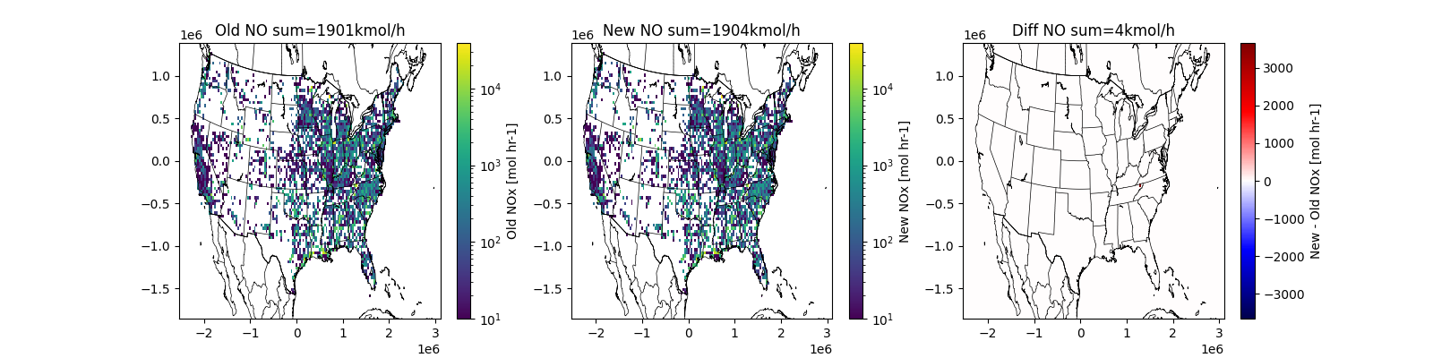
Visualize Source to confirm operational

• Create gridded data for quick visualiation

• Show new, original and difference.

import matplotlib.colors as mc
import matplotlib.pyplot as plt
import pycno
import numpy as np

oldf = netCDF4.Dataset(oldpath, mode='r')
newf = netCDF4.Dataset(newpath, mode='r')

x = oldf['xcoord'][:]
y = oldf['ycoord'][:]
# add all emission keys
zold = sum([oldf[ek][:].mean(0) for ek in scalekeys])
znew = sum([newf[ek][:].mean(0) for ek in scalekeys])

xedges = np.arange(0.5, oldf.NCOLS) * oldf.XCELL + oldf.XORIG
yedges = np.arange(0.5, oldf.NROWS) * oldf.YCELL + oldf.YORIG
Hold, _, _ = np.histogram2d(y, x, weights=zold, bins=[yedges, xedges])
Hnew, _, _ = np.histogram2d(y, x, weights=znew, bins=[yedges, xedges])

gskw = dict(left=0.333, right=0.967)
fig, axx = plt.subplots(1, 3, figsize=(16, 4))
opts = dict(norm=mc.LogNorm(10), cmap='viridis')
qm = axx[0].pcolormesh(xedges, yedges, Hold, **opts)
fig.colorbar(qm, label='Old NOx [mol hr-1]')
axx[0].set(title=f'Old NO sum={Hold.sum() / 1e3:.0f}kmol/h')
qm = axx[1].pcolormesh(xedges, yedges, Hnew, **opts)
fig.colorbar(qm, label='New NOx [mol hr-1]')
axx[1].set(title=f'New NO sum={Hnew.sum() / 1e3:.0f}kmol/h')
opts['norm'] = mc.TwoSlopeNorm(0)
opts['cmap'] = 'seismic'
qm = axx[2].pcolormesh(xedges, yedges, Hnew - Hold, **opts)
fig.colorbar(qm, label='New - Old NOx [mol hr-1]')
axx[2].set(title=f'Diff NO sum={(Hnew.sum() - Hold.sum()) / 1e3:.0f}kmol/h')
pycno.cno(proj=proj).drawstates(resnum=1, ax=axx)

fig.savefig(figpath)

Extra Credit

1. Modify the custom section to scale all point sources in your home state.

2. Modify the custom section to scale all point sources in the counties in a nonattainment area.