Compare Model to Daily MDA8 Observations

Evaluate CAMx by comparing to AirNow or AQS Ozone observations using the 2015 Ozone NAAQS definition of the maximum daily 8-hour average metric.

The basic steps are:

1. Open CAMx file and identify space/time domain,

2. Download hourly observations for that domain to a CSV file.

3. Add CAMx hourly model data to the observations CSV file.

4. Apply Maximum Daily 8-hour average (Appendix U).

5. Calculate statistics.

6. Plot a time series

Reminder: You must have already activated your python environment.

Configuration

# Define Analysis
obssrc = 'airnow'  # or aqs
obsspc = 'ozone'     # or ozone, co, pm25, ...
modsrc = 'CAMx'    # Or CMAQ
modspc = 'O3'     # or O3, CO, PM25, ...

# Set input files
dates = ['20160610', '20160611']
avrgtmpl = '../../camx/outputs/CAMx.v7.32.36.12.{}.avrg.grd02.nc'  # placeholder {} for date

# Outputs
outstem = f'outputs/{obssrc}.{obsspc}_MDA8_and_CAMx.v7.32.36.12.avrg.grd02'
pairedpath = outstem + '.csv'
statspath = outstem + '_stats.csv'
figpath = outstem + '_ts.png'

Imports and Folders

import pyrsig
import pandas as pd
import matplotlib.pyplot as plt
import os

os.makedirs('outputs', exist_ok=True)

Query Observations for Model file

obskey = f'{obssrc}.{obsspc}'  # must exist in RSIG
modkey = f'{modsrc}{modspc}'
keys = [obskey, modkey]
dfs = []
for datestr in ['20160610', '20160611']:
    ncpath = f'../../camx/outputs/CAMx.v7.32.36.12.{datestr}.avrg.grd02.nc'
    ds = pyrsig.open_ioapi(ncpath)
    df = pyrsig.cmaq.pair_rsigcmaq(ds, modspc, obskey, prefix=modsrc, workdir='outputs')
    df[modkey] *= 1000
    df.rename(columns={obsspc: obskey}, inplace=True)
    dfs.append(df)

df = pd.concat(dfs)

Using cached: outputs/airnow.ozone_2016-06-10T000000Z_2016-06-10T235959Z.csv.gz
Using cached: outputs/airnow.ozone_2016-06-11T000000Z_2016-06-11T235959Z.csv.gz

Calculate Hourly Statistics

statsdf = pyrsig.utils.quickstats(df[keys], obskey)
# Save stats to disk
statsdf.to_csv(statspath)
print(statsdf)

       airnow.ozone        CAMxO3
count  29892.000000  29892.000000
mean      38.099505     41.653587
std       19.807133     12.087435
min        0.000000      0.301045
25%       22.665580     33.589913
50%       38.000000     42.133999
75%       53.100000     49.821673
max      115.000000    110.212502
r          1.000000      0.698374
mb         0.000000      3.554083
nmb        0.000000      0.093284
fmb        0.000000      0.089127
ioa        1.000000      0.772703

40 CFR Appendix U to Part 50

• 3(a) hourly data in LST truncated to ppb precision

• 3(b) minimum of 6 valid hourly values for an 8h average

• 3(c) 17 possible valid 8h LST windows per day (07-15 LST, …, 23-07 LST)

• 3(d) a daily maximum is valid if 13 of 17 possible windows available

https://www.ecfr.gov/current/title-40/chapter-I/subchapter-C/part-50/

Step 3(a): Adjust Times to LST

• Get timezone from latitude

• Convert tz-aware UTC to tz-naive LST

• not truncating

tz = (df.groupby('STATION')['LONGITUDE'].mean() / 15).round(0)
tz = pd.to_timedelta(tz, unit='h')  # EST=-5h, ... PST=-8h
df['time_lst'] = df['time'].dt.tz_convert(None) + tz.loc[df.STATION].values

Step 3(b): Calculate 8h averages

for each site: 1. regularize to hourly data with missing nans 2. create 8h averages only valid when 6 or more available

a8df = df[['STATION', 'time_lst', obskey, modkey]].groupby('STATION').apply(
    lambda sdf:
    sdf.set_index('time_lst')[[obskey, modkey]].asfreq('1h')
    .rolling('8h', min_periods=6).mean(),
    include_groups=True
)

/work/ROMO/users/bhenders/SESARMTraining/examples/mpe/run_mpe_02_o3mda8.py:106: FutureWarning: DataFrameGroupBy.apply operated on the grouping columns. This behavior is deprecated, and in a future version of pandas the grouping columns will be excluded from the operation. Either pass `include_groups=False` to exclude the groupings or explicitly select the grouping columns after groupby to silence this warning.
  a8df = df[['STATION', 'time_lst', obskey, modkey]].groupby('STATION').apply(

Step 3(c): Calculate 8h averages

Pandas labels 8h means based on start time in LST 1. regularize to hourly data with missing nans 2. remove 00-06 LST hours that duplicate previous day’s hours

# pandas labels the first 8h average (hours 00-07) as 07, so decrement
# the start_time_lst hour by 7h to match starting time
iddf = a8df.index.to_frame()
iddf['start_time_lst'] = iddf['time_lst'] + pd.to_timedelta('-7h')
a8df.index = pd.MultiIndex.from_frame(iddf[['STATION', 'start_time_lst']])
# Valid if 13 of 17 possible valid windows (07-15 LST, ..., 23-07 LST)
# Remove the 8h averages starting 00-06 LST
n = a8df.shape[0]
a8df.query('start_time_lst.dt.hour > 6', inplace=True)
nnew = a8df.shape[0]
print(f'INFO:: removed {n - nnew} ({1 - nnew / n:.2%}) 8h avg (7 morning hours)')

INFO:: removed 8954 (29.19%) 8h avg (7 morning hours)

Step 3(d): Calculate daily maxima

For each STATION, - get the max 8h average within a local standard day - remove when fewer than 13 available

mda8df = a8df.groupby(['STATION', pd.Grouper(level='start_time_lst', freq='24h')]).agg(**{
    obskey: (obskey, 'max'),
    modkey: (modkey, 'max'),
    'count': (obskey, 'count')
})
n = mda8df.shape[0]
mda8df.query('count >= 13', inplace=True)
nnew = mda8df.shape[0]
print(f'INFO:: removed {n - nnew} ({1 - nnew / n:.2%}) MDA8 values (less than 13 8h avgs)')
mda8df['COUNTYFP'] = mda8df.index.to_frame()['STATION'].astype(str).str[:5]
mda8df.to_csv(pairedpath)

INFO:: removed 1320 (68.75%) MDA8 values (less than 13 8h avgs)

Calculate MDA8 Statistics

statsdf = pyrsig.utils.quickstats(mda8df[keys], obskey)
# Save stats to disk
statsdf.to_csv(statspath)
# Print them for the user to review.
print(statsdf)

       airnow.ozone      CAMxO3
count    600.000000  600.000000
mean      52.517737   51.605904
std       17.265956   11.977870
min       13.462500   24.430573
25%       41.718750   44.530444
50%       55.906250   53.408267
75%       64.856250   59.050945
max      105.625000   99.977543
r          1.000000    0.868137
mb         0.000000   -0.911833
nmb        0.000000   -0.017362
fmb        0.000000   -0.017514
ioa        1.000000    0.897360

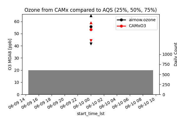
Visualize Results

gb = mda8df.groupby('start_time_lst')[keys]
cntdf = gb.count().reset_index()

fig, ax = plt.subplots(figsize=(6, 4))
tax = ax.twinx()
x = cntdf['start_time_lst'].to_numpy()
tax.bar(x=x, height=cntdf[modkey], color='pink')
tax.bar(x=x, height=cntdf[obskey], color='grey')
gb.median().plot(color=['k', 'r'], linewidth=2, zorder=2, ax=ax, marker='o')
gb.quantile(.75).plot(ax=ax, color=['k', 'r'], linestyle='--', legend=False, zorder=1, marker='^')
gb.quantile(.25).plot(ax=ax, color=['k', 'r'], linestyle='--', legend=False, zorder=1, marker='v')
tax.set(zorder=0, facecolor='w', ylim=(0, 2000), yticks=[0, 250, 500, 750, 1000])
tax.set(ylabel='Daily Count')
ax.set(zorder=1, facecolor='none', ylim=(0, None), ylabel='O3 MDA8 [ppb]')
ax.set(title='Ozone from CAMx compared to AQS (25%, 50%, 75%)')
fig.savefig(figpath)

Extra Credit

1. Modify the script to evaulate 1-hour maximum hourly ozone.

2. Modify the script to evaluate W126.