Region-specific Gridded Emission Scaling

Apply a constant factor to selected emission variables within a region.The region can be as simple as a rectangular box, a circle, or any geographic shape you can define.

The basic steps are:

1. Copy a file.

2. Select species to scale NOx species.

3. Define a region of application.

4. Scale by a multiplicative factor.

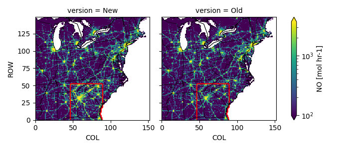
5. Plot the old and new result.

Reminder: You must have already activated your python environment.

Configuration

# date to process
date = '20160610'
# file to use as input
oldpath = f'../../camx/emiss/camx_area.mobile.{date}.12km.nc'
# file to create
newpath = f'outputs/camx_area_2x_county.mobile.{date}.12km.nc'

# species to scale
scalekeys = ['NO', 'NO2', 'HONO']  # list of strings or set to 'all'
# factor to scale by
factor = 2.
# bounding box within which to scale
bbox = [-86.5, 30, -80, 35.5]      # [wlon,slat,elon,nlat] or 'custom'

# figure demonstrating the change
figpath = 'outputs/scaled_gridemiss_scaleregion.png'

Imports and File Prep

import shutil
import os
import numpy as np
import netCDF4
import pyproj
from shapely import points, box

os.makedirs('outputs', exist_ok=True)
shutil.copyfile(oldpath, newpath)

'outputs/camx_area_2x_county.mobile.20160610.12km.nc'

Open Files

• Open the existing file in read-only mode

• Open the new file in editable append mode

oldfile = netCDF4.Dataset(oldpath, mode='r')
newfile = netCDF4.Dataset(newpath, mode='a')

Select Emission Variables to Scale

if scalespecies is all, identify emission variables by unit

if scalekeys == 'all':
    # Find all emission variables
    scalekeys = [
        k for k, v in newfile.variables.items()               # for all key/variable pairs
        if v.units.strip().lower() in ('mol hr-1', 'g hr-1')  # if has emission units
    ]

noscalekeys = sorted(set(newfile.variables).difference(scalekeys))
print('INFO:: no scale', noscalekeys)
print('INFO:: to scale', scalekeys)

INFO:: no scale ['ACET', 'ALD2', 'ALDX', 'BENZ', 'BNZA', 'CH4', 'CO', 'CPRM', 'ECH4', 'ETFLAG', 'ETH', 'ETHA', 'ETHY', 'ETOH', 'FORM', 'FPRM', 'IOLE', 'ISOP', 'ISP', 'IVOA', 'KET', 'MEOH', 'NA', 'NH3', 'NVOL', 'OLE', 'PAL', 'PAR', 'PCA', 'PCL', 'PEC', 'PFE', 'PH2O', 'PK', 'PMG', 'PMN', 'PNH4', 'PNO3', 'POA', 'PRPA', 'PSI', 'PSO4', 'PTI', 'SO2', 'SULF', 'TERP', 'TFLAG', 'TOL', 'TOLA', 'TRP', 'UNK', 'UNR', 'X', 'XYL', 'Y', 'latitude', 'longitude']
INFO:: to scale ['NO', 'NO2', 'HONO']

Define Emission Coordinates

• define a projection based on file metadata,

• define coordinates for cell centroids

# define projection
attrs = {k: oldfile.getncattr(k) for k in oldfile.ncattrs()}
proj4tmpl = '+proj=lcc +lat_0={YCENT} +lon_0={P_GAM}'
proj4tmpl += ' +lat_1={P_ALP} +lat_2={P_BET} +R=6370000 +units=m +no_defs'
proj4str = proj4tmpl.format(**attrs)
proj = pyproj.Proj(proj4str)

# Calculate grid cell centroid coordinates
# approximately X * 1000, but more precise
x = np.arange(0.5, oldfile.NCOLS) * oldfile.XCELL + oldfile.XORIG  # x(COL)
# approximately Y * 1000, but more precise
y = np.arange(0.5, oldfile.NROWS) * oldfile.YCELL + oldfile.YORIG  # y(ROW)
X, Y = np.meshgrid(x, y)  # X(ROW, COL), Y(ROW, COL)

Define an area for scaling

• define a projected box of interest,

• optionally, define a complex area from US Census shapefile

# simple longitude/latitude bounding box from corners
if bbox != 'custom':
    pbbox = proj(*bbox[:2]) + proj(*bbox[2:])
    myshp = box(*pbbox)
else:
    # More complex based on counties from US Census
    import geopandas as gpd

    # downloaded from census.gov
    cntypath = '../../www2.census.gov/geo/tiger/TIGER2020/COUNTY/tl_2020_us_county.zip'
    cnty = gpd.read_file(cntypath, bbox=(-135, 20, -60, 60))

    # Select counties in Georgia, reproject to grid space, collapse to one big shape (i.e, state)
    myshp = cnty.query('STATEFP == "13"').to_crs(proj.srs).union_all()

    # Select DeKalb county in Georgia, reproject to grid space, collapse to one shape
    # myshp = cnty.query('GEOID == "13091"').to_crs(proj.srs).union_all()

gcxy = points(X, Y)
ismine = myshp.intersects(gcxy)
print(f'INFO:: found {ismine.sum()} cells with centroids in the myshp')

INFO:: found 2184 cells with centroids in the myshp

Define Scaling Factor

factor = np.where(ismine, factor, 1)

print(f'INFO:: factor min={factor.min():.3e}')
print(f'INFO:: factor avg={factor.mean():.3e}')
print(f'INFO:: factor std={factor.std():.3e}')
print(f'INFO:: factor max={factor.max():.3e}')

INFO:: factor min=1.000e+00
INFO:: factor avg=1.096e+00
INFO:: factor std=2.952e-01
INFO:: factor max=2.000e+00

Apply Scaling

for skey in scalekeys:
    print('INFO:: scaling', skey)
    outvar = newfile[skey]
    invar = oldfile[skey]
    outvar[:] = factor * invar[:]

newfile.sync()
del newfile

INFO:: scaling NO
INFO:: scaling NO2
INFO:: scaling HONO

Plot Comparison

import pyrsig
import pycno
import matplotlib.colors as mc

oldfile = pyrsig.open_ioapi(oldpath)
newfile = pyrsig.open_ioapi(newpath)

key = scalekeys[0]
compfile = newfile[[]]
compfile['New'] = newfile[key].sum('LAY').mean('TSTEP')
compfile['Old'] = oldfile[key].sum('LAY').mean('TSTEP')
Z = compfile.to_dataarray(dim='version')
Z.attrs.update(oldfile[key].attrs)
fca = Z.plot(col='version', norm=mc.LogNorm(100, compfile['Old'].quantile(.995)))

bboxx = pbbox[0], pbbox[2], pbbox[2], pbbox[0], pbbox[0]
bboxy = pbbox[1], pbbox[1], pbbox[3], pbbox[3], pbbox[1]

dZ = np.abs(compfile['New'] - compfile['Old'])
for ax in fca.axs.ravel():
    dZ.plot.contour(levels=[0], colors=['r'], ax=ax, add_labels=False)


pycno.cno(oldfile.crs_proj4).drawstates(ax=fca.axs)
fca.fig.savefig(figpath)

Extra Credit

1. Modify the custom section to scale all point sources in your home state.

2. Modify the custom section to scale all point sources in the counties in a nonattainment area.