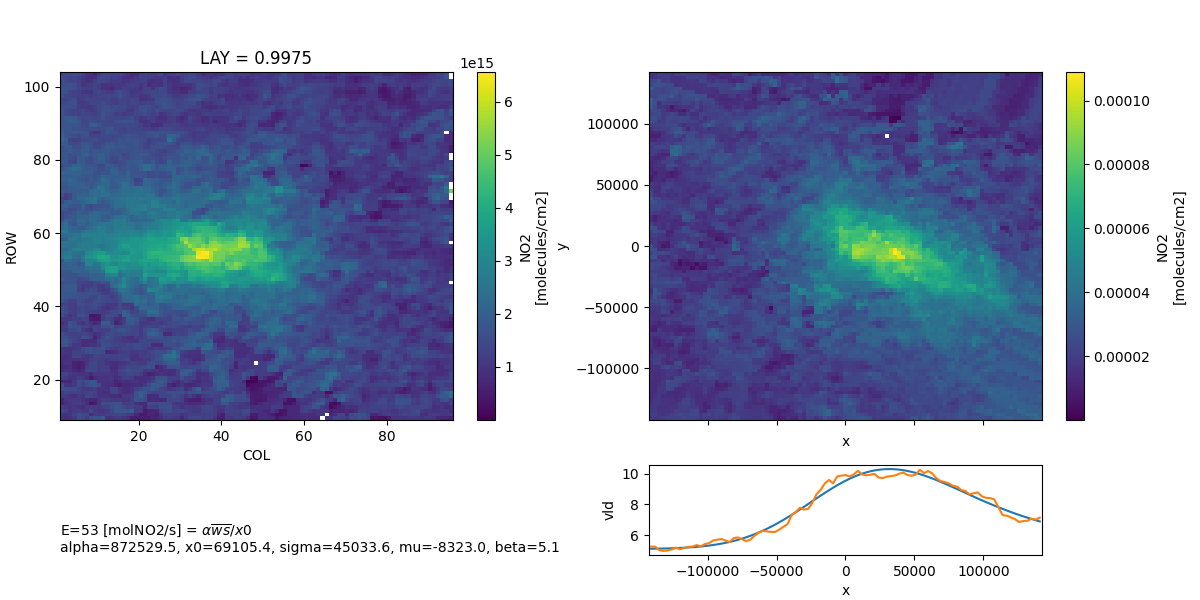
Calculate Emissions by Fitting a Modified Guassian

This example uses Dallas Fort Worth Texas as an illustrative application of this technique. For illustration, only 3 days are used. In practice, it should use as whole year or the ozone season to get a more robust estimate.

Steps: 1. Create a 3km custom L3 product on the HRRR grid, 2. Retrieve HRRR winds at center of domain, 3. Rotate daily rasters so that wind blows from left to right, 4. Fit Eq 1 of Goldberg et al. (10.5194/acp-22-10875-2022; ~exponnorm), 5. Derive tau parameter and estimate emissions.

The 4 day result 41 moles/s, which is in good agreement with the 2017 NEI[1,2] 60870 short-tons/yr (38 moles/s) and larger than the 2020 NEI[3,4] 47110 short- tons/yr (29 moles/s).

These days were selected because of the reasonable agreement. In actual application, you should check the rotation of each day and apply to many days. The alignment of winds with plumes is imperfect due to meandering winds.

[1] https://enviro.epa.gov/envirofacts/embed/nei?pType=TIER&pReport=county&pState=&pState=48&pPollutant=&pPollutant=NOX&pSector=&pYear=2017&pCounty=48439&pTier=&pWho=NEI [2] https://enviro.epa.gov/envirofacts/embed/nei?pType=TIER&pReport=county&pState=&pState=48&pPollutant=&pPollutant=NOX&pSector=&pYear=2017&pCounty=48113&pTier=&pWho=NEI [3] https://enviro.epa.gov/envirofacts/embed/nei?pType=TIER&pReport=county&pState=&pState=48&pPollutant=&pPollutant=NOX&pSector=&pYear=2020&pCounty=48439&pTier=&pWho=NEI [4] https://enviro.epa.gov/envirofacts/embed/nei?pType=TIER&pReport=county&pState=&pState=48&pPollutant=&pPollutant=NOX&pSector=&pYear=2020&pCounty=48113&pTier=&pWho=NEI

import matplotlib.pyplot as plt
import numpy as np
import pyrsig
import pandas as pd

Define Location and Date Range

• Location is a single point

• Date range can be a few days at a time

• vbbox is the box to retrieve VCDs

workdir = 'dfw'
loc = (-96.95, 32.85)
dates = pd.date_range('2023-05-01T00Z', '2023-05-04T00Z', freq='1d')
vbbox = np.array(loc + loc) + np.array([-1, -1, 1, 1]) * 1.5

Get TropOMI NO2 Over vbbox

vrsig = pyrsig.RsigApi(
    bbox=vbbox, workdir=workdir, grid_kw='HRRR3K', gridfit=True
)
vkey = 'tropomi.offl.no2.nitrogendioxide_tropospheric_column'
ds = vrsig.to_ioapi(bdate=dates, key=vkey)

# Make the output square by windowing in on the center
n = min(ds.sizes['COL'], ds.sizes['ROW'])
n = n - 1 if n % 2 == 0 else n
dn = n / 2
mc = ds.COL.mean().astype('i') + 0.5  # Get nearest cell center
mr = ds.ROW.mean().astype('i') + 0.5  # Get nearest cell center
ds = ds.sel(ROW=slice(mr - dn, mr + dn), COL=slice(mc - dn, mc + dn))
# removing missing values
ds = ds.where(lambda x: x > -9e30)

Get Winds At Domain Center

• Find the domain center

• Create a 0.01 degree box around it

• retrieve the HRRR 80m wind components (requires xdr)

# Find the center lon/lat to query for wind speed
llds = ds.isel(TSTEP=0, LAY=0).sel(ROW=ds.ROW.mean(), COL=ds.COL.mean(), method='nearest')
wloc = float(llds.LONGITUDE), float(llds.LATITUDE)
wbbox = np.array(wloc + wloc) + np.array([-1, -1, 1, 1]) * .005
wrsig = pyrsig.RsigApi(bbox=wbbox, workdir=workdir)
wkey = 'hrrr.wind_80m'
df = wrsig.to_dataframe(bdate=dates, key=wkey, unit_keys=False, parse_dates=True, backend='xdr')
df = df.loc[df['time'].dt.tz_convert(None).isin(ds.TSTEP.data)]  # only if a valid record is avail

# Add wind components to the VCD dataset
ds['wind_80m_u'] = ('TSTEP',), df.wind_80m_u.values, dict(units='m/s')
ds['wind_80m_v'] = ('TSTEP',), df.wind_80m_v.values, dict(units='m/s')

Fit Exponential Modified Gaussian

• Convert from molecules/cm2 to mole/m2

• Fit using u/v wind components and the width of cells in m

molperm2 = ds.NO2 / 6.022e23 * 1e4
dxm = ds.XCELL
emgout = pyrsig.emiss.fitemg(molperm2, ds.wind_80m_u, ds.wind_80m_v, dx=dxm)
emgout['wind_80m_u'] = ('time',), ds.wind_80m_u.data
emgout['wind_80m_v'] = ('time',), ds.wind_80m_v.data
emgout.to_netcdf(f'{workdir}/emg.nc')

Plot EMG Result and Derived Props

• Create a 3-panel plot (unrotated VCD mean, rotated VCD mean and VLD)

• Fit using u/v wind components and the width of cells in m

gskw = dict(left=0.05, right=0.95, bottom=0.3)
fig, axx = plt.subplots(1, 2, figsize=(12, 6), gridspec_kw=gskw)
axw = .9 / 2.1
ds.NO2.mean('TSTEP').plot(ax=axx[0])
emgout.ROTATED_VCD.mean('time').plot(ax=axx[1])
bbox = axx[1].get_position()
bbox.y0 = 0.075
bbox.y1 = 0.225
axx[1].xaxis.set_major_formatter(plt.matplotlib.ticker.NullFormatter())
inax = fig.add_axes(bbox)
emgout.vldhat.plot(ax=inax)
emgout.vld.plot(ax=inax)
inax.set_xticks(axx[1].get_xticks())
inax.set_xlim(axx[1].get_xlim())
tag = ', '.join([f'{k}={v:.1f}' for k, v in emgout.vldhat.attrs.items()])
tag = f'E={emgout.emis_no2:.0f} [{emgout.emis_no2.units}] = $\\alpha \\overline{{ws}} / x0$\n{tag}'
fig.text(0.05, 0.075, tag, ha='left', va='bottom')
figpath = f'{workdir}/emg.png'
fig.savefig(figpath)
# Requires geopandas to add county and primary roads
try:
    import geopandas as gpd
    cntypath = 'https://www2.census.gov/geo/tiger/TIGER2023/COUNTY/tl_2023_us_county.zip'
    cnty = gpd.read_file(cntypath, bbox=tuple(vbbox)).to_crs(ds.crs_proj4)
    roadpath = 'https://www2.census.gov/geo/tiger/TIGER2023/PRIMARYROADS/tl_2023_us_primaryroads.zip'
    road = gpd.read_file(roadpath, bbox=tuple(vbbox)).to_crs(ds.crs_proj4)
    cnty.plot(facecolor='none', edgecolor='gray', linewidth=.6, ax=axx[0])
    road.plot(facecolor='none', edgecolor='gray', linewidth=.3, ax=axx[0])
    fig.savefig(figpath)
except Exception as e:
    print('failed to add map', str(e))

/opt/hostedtoolcache/Python/3.13.7/x64/lib/python3.13/site-packages/pyogrio/raw.py:198: RuntimeWarning: HTTP response code on https://www2.census.gov/geo/tiger/TIGER2023/COUNTY/tl_2023_us_county.zip: 0
  return ogr_read(
failed to add map '/vsizip/vsicurl/https://www2.census.gov/geo/tiger/TIGER2023/COUNTY/tl_2023_us_county.zip' does not exist in the file system, and is not recognized as a supported dataset name.