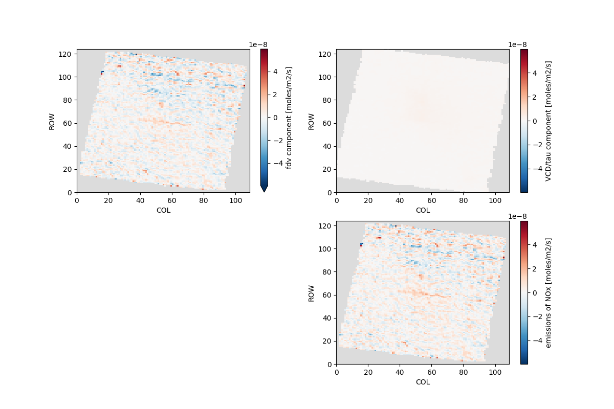
Calculate Emissions by Flux Divergence

This example uses Phoenix Arizona to illustrate the flux-divergence technique. As an illustration, it is oversimplified to use just 4 days, and should be extended to a whole year to get a more robust estimate. Further, the value of tau is simply assumed. These elements would need more work before application.

Steps: 1. Create a 3km custom L3 NO2 product on the HRRR grid, 2. Retrieve HRRR winds at cell centers for the same domain, 3. Fit Eq 3 of Goldberg et al. (10.5194/acp-22-10875-2022), 4. Assume a plausible tau parameter and estimate emissions.

Application from 2023-05-01 to 2023-05-04 with a 6h lifteime (tau=6h) yields a Maricopa annualized emission rate of 47.2 GgNO2/yr. This value is higher than the NEI 2020[1] reported 43668 short tons (39.6 GgNO2/yr) and lower than the NEI 2017[2] value of 59891 short tons (54.3 GgNO2/yr).

Extending to this application to the whole 2023 year yields 49.6 GgNO2/yr. And, there are many sensitivities that one can test with respect to sampling time. Further, the results are very sensitive to the assumed value of tau which is not spatially constant or well known.

[1] https://enviro.epa.gov/envirofacts/embed/nei?pType=TIER&pReport=county&pState=&pState=04&pPollutant=&pPollutant=NOX&pSector=&pYear=2020&pCounty=04013&pTier=&pWho=NEI [2] https://enviro.epa.gov/envirofacts/embed/nei?pType=TIER&pReport=county&pState=&pState=04&pPollutant=&pPollutant=NOX&pSector=&pYear=2017&pCounty=04013&pTier=&pWho=NEI

import matplotlib.pyplot as plt
import numpy as np
import pyrsig
import pandas as pd
import xarray as xr

Define Location and Date Range

• Location is a single point

• Date range can be a few days at a time

• bbox is the box to retrieve VCDs

cntyname = 'Maricopa'
loc = (-112.0777, 33.4482)  # Phoenix Arizona - fit is not good due to multiple loci
# cntyname = 'Harris'
# loc = (-95.1, 29.720621)  # Houston Texas
dates = pd.date_range('2023-05-01T00Z', '2023-05-04T00Z', freq='1d')
bbox = np.array(loc + loc) + np.array([-1, -1, 1, 1]) * 1.5
tauh = 6

Get TropOMI NO2 Over bbox

rsig = pyrsig.RsigApi(
    bbox=bbox, workdir=cntyname, grid_kw='HRRR3K', gridfit=True
)
vkey = 'tropomi.offl.no2.nitrogendioxide_tropospheric_column'
ds = rsig.to_ioapi(bdate=dates, key=vkey)

# removing missing values
ds = ds.where(lambda x: x > -9e30)

Get Winds Across Domain

• retrieve the HRRR 80m wind components

wkey = 'hrrr.wind_80m'
wds = rsig.to_ioapi(bdate=dates, key=wkey).where(lambda x: x > -9e30)
wds = wds.sel(TSTEP=ds.TSTEP)
# Add wind components to the VCD dataset
ds['WIND_80M_U'] = wds['wind_80m_u'].dims, wds['wind_80m_u'].data
ds['WIND_80M_V'] = wds['wind_80m_v'].dims, wds['wind_80m_v'].data

Calculate the Column Divergence

ds['DCDX'] = ds['NO2'] * np.nan
ds['DCDY'] = ds['NO2'] * np.nan
for ti, t in enumerate(ds.TSTEP.dt.strftime('%FT%HZ').values):
    print(t)
    v = ds['NO2'][ti, 0]
    if not v.isnull().all():
        dcdx, dcdy = pyrsig.emiss.divergence(v.data, ds.XCELL, ds.YCELL, withdiag=False)
        ds['DCDX'][ti, 0] = dcdx
        ds['DCDY'][ti, 0] = dcdy

2023-05-01T00Z
2023-05-01T01Z
2023-05-01T02Z
2023-05-01T03Z
2023-05-01T04Z
2023-05-01T05Z
2023-05-01T06Z
2023-05-01T07Z
2023-05-01T08Z
2023-05-01T09Z
2023-05-01T10Z
2023-05-01T11Z
2023-05-01T12Z
2023-05-01T13Z
2023-05-01T14Z
2023-05-01T15Z
2023-05-01T16Z
2023-05-01T17Z
2023-05-01T18Z
2023-05-01T19Z
2023-05-01T20Z
2023-05-01T21Z
2023-05-01T22Z
2023-05-01T23Z
2023-05-02T00Z
2023-05-02T01Z
2023-05-02T02Z
2023-05-02T03Z
2023-05-02T04Z
2023-05-02T05Z
2023-05-02T06Z
2023-05-02T07Z
2023-05-02T08Z
2023-05-02T09Z
2023-05-02T10Z
2023-05-02T11Z
2023-05-02T12Z
2023-05-02T13Z
2023-05-02T14Z
2023-05-02T15Z
2023-05-02T16Z
2023-05-02T17Z
2023-05-02T18Z
2023-05-02T19Z
2023-05-02T20Z
2023-05-02T21Z
2023-05-02T22Z
2023-05-02T23Z
2023-05-03T00Z
2023-05-03T01Z
2023-05-03T02Z
2023-05-03T03Z
2023-05-03T04Z
2023-05-03T05Z
2023-05-03T06Z
2023-05-03T07Z
2023-05-03T08Z
2023-05-03T09Z
2023-05-03T10Z
2023-05-03T11Z
2023-05-03T12Z
2023-05-03T13Z
2023-05-03T14Z
2023-05-03T15Z
2023-05-03T16Z
2023-05-03T17Z
2023-05-03T18Z
2023-05-03T19Z
2023-05-03T20Z
2023-05-03T21Z
2023-05-03T22Z
2023-05-03T23Z
2023-05-04T00Z
2023-05-04T01Z
2023-05-04T02Z
2023-05-04T03Z
2023-05-04T04Z
2023-05-04T05Z
2023-05-04T06Z
2023-05-04T07Z
2023-05-04T08Z
2023-05-04T09Z
2023-05-04T10Z
2023-05-04T11Z
2023-05-04T12Z
2023-05-04T13Z
2023-05-04T14Z
2023-05-04T15Z
2023-05-04T16Z
2023-05-04T17Z
2023-05-04T18Z
2023-05-04T19Z
2023-05-04T20Z
2023-05-04T21Z
2023-05-04T22Z
2023-05-04T23Z

Multiply by Orthogonal Wind Components

ds['FDV'] = ds['DCDX'] * ds['WIND_80M_U'] + ds['DCDY'] * ds['WIND_80M_V']
ds['FDV'].attrs.update(
    long_name='column divergence',
    description='div(V w) = dV/dx*u + dV/dy*v',
    units='molecules/cm2/s'
)

Add Chemical Lifetime Correction for Emissions

• tau is a simple assumption of 6h, but should be improved for specific application by allowing it to vary in space and time.

• Units are converted to moles/m2/s for more common representation

tau = tauh * 3600  # s
N_A = 6.022e23
A = ds.XCELL * ds.YCELL
# convert from moleculesNO2/cm2/s to molesNOx/m2/s
fdvNOx = ds['FDV'] / N_A * 1e4 * 1.32
fdvNOx.attrs.update(
    long_name='fdv component',
    description='div(V w) * 1.32',
    units='moles/m2/s'
)
tauNOx = ds['NO2'] / tau / N_A * 1e4 * 1.32
tauNOx.attrs.update(
    long_name='VCD/tau component',
    description='V / tau * 1.32',
    units='moles/m2/s'
)
eNOx = fdvNOx + tauNOx
eNOx.attrs.update(
    long_name='emissions of NOx',
    description='(div(V w) + V / tau) * 1.32',
    units='moles/m2/s'
)
ds['emiss_nox'] = eNOx
outds = ds[['FDV', 'emiss_nox']]
outds.attrs.update(ds.attrs)
outds.to_netcdf(f'{cntyname}/flux.nc')

Plot Emission Results

• Create a simple plot of emissions

• Then intersect cells with Maricopa county and sum for county total

fig, axx = plt.subplots(2, 2, figsize=(12, 8))
plt.setp(axx, facecolor='gainsboro')
figpath = f'{cntyname}/flux.png'

# Requires geopandas to add county and primary roads
try:
    import geopandas as gpd
    import shapely
    cntypath = 'https://www2.census.gov/geo/tiger/TIGER2023/COUNTY/tl_2023_us_county.zip'
    roadpath = 'https://www2.census.gov/geo/tiger/TIGER2023/PRIMARYROADS/tl_2023_us_primaryroads.zip'
    cnty = gpd.read_file(cntypath, bbox=tuple(bbox)).to_crs(ds.crs_proj4)
    r, c = xr.broadcast(eNOx.ROW, eNOx.COL)
    cntypoly = cnty.query(f'NAME == "{cntyname}"').unary_union
    incnty = cntypoly.contains(shapely.points(np.stack([c, r], axis=-1)))  # Is each cell in Maricopa?
    incnty = xr.DataArray(incnty, dims=('ROW', 'COL'))
    fdvNOx = fdvNOx.where(incnty)
    tauNOx = tauNOx.where(incnty)
    eNOx = eNOx.where(incnty)
    massrate_nox = eNOx.mean(('TSTEP', 'LAY')).sum() * ds.XCELL * ds.YCELL * 46.  # moles/m2/s to gNO2/s
    mass = massrate_nox / 1e9 * 365 * 24 * 3600  # gNO2/s to Gg/yr
    label = f'{cntyname} ENOx = {mass:.1f} [GgNO2/yr]'
    print(label)
    road = gpd.read_file(roadpath, bbox=tuple(bbox)).to_crs(ds.crs_proj4)
    for ax in axx.ravel():
        cnty.plot(facecolor='none', edgecolor='gray', linewidth=.6, ax=ax, zorder=2)
        road.plot(facecolor='none', edgecolor='gray', linewidth=.3, ax=ax, zorder=2)
    ax.text(0.05, 0.975, label, transform=ax.transAxes, va='top')
except Exception as e:
    print('failed to add map', str(e))

qm = eNOx.mean(('TSTEP', 'LAY')).plot(ax=axx[1, 1], zorder=1)
fdvNOx.mean(('TSTEP', 'LAY')).plot(ax=axx[0, 0], norm=qm.norm, cmap=qm.cmap, zorder=1)
tauNOx.mean(('TSTEP', 'LAY')).plot(ax=axx[0, 1], norm=qm.norm, cmap=qm.cmap, zorder=1)
axx[1, 0].set(visible=False)
fig.savefig(figpath)

failed to add map '/vsizip/vsicurl/https://www2.census.gov/geo/tiger/TIGER2023/COUNTY/tl_2023_us_county.zip' does not exist in the file system, and is not recognized as a supported dataset name.