Pairing Population with Concentration

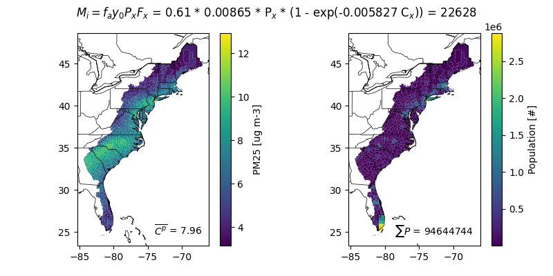
This example performs a simple health benefit assessment by pairing model concentrations with population datasets in RSIG. The population dataset comes from the Integrated Climate and Land Use Scenarios (ICLUS). The concentration dataset comes from the EPA’s Air QUAlity TimE Series Project (EQUATES) project. The concentration response function (CRF) uses Krewski 2009.

Conceptualy, mortality or morbitidy (M) is attributed to cause (i) based on an attributable fraction (F) as a function of space (x). For air quality applications, the F_x is a function of pollutant concentrations or mixing ratios. Often, M_x is known at a coarser spatial resolution than is ideal. In that case, M_x may be translated into a fractional baseline incidence (y0_x) and used to estimate M_x using spatially resolved P_x.

m_x = M_x * F_x = y0_x * P_x * F_x

In this example, the problem is (over)simplified in three ways: 1. Mortality is applied at the county-level assuming no intracounty variation. 2. It assumes the age-stratification is nationally homogenous. 3. It assumes that baseline incidence is nationally homogenous.

The example datasets and CRF can be replaced. The geopandas package read_file function can be used to open shapefiles with M_x at polygons. So, you could create age-specific mortality incidence at census tract level to improve this example.

import matplotlib.pyplot as plt
import numpy as np
import pandas as pd
import xarray as xr
from shapely import polygons
import geopandas as gpd
import pycno
import pyrsig


datakey = 'cmaq.equates.conus.aconc.PM25'
ckey = 'PM25'

Concentration Reponse Function Formulation

• Krewski 2009 PM25 * all-cause mortality risk 1.06 per 10 micrograms/m3 * 30+ year-old population

• Simplifying Assumptions * Baseline mortality incidence is spatiall uniform

  • [GDB IHME](vizhub.healthdata.org/gbd-results) for 2019 in the US

  • all cause deaths = 2853165.03

  • population = 329996155.19

  • Age distribution is spatially unfiorm * Age distribution from the US Census ACSST5Y2020 * US population 30 years or older: 201686433 * US population total : 329824950

beta = np.log(1.06) / 10
y0 = 2853165.03 / 329996155.19
f_pop = 201686433 / 329824950


bdates = pd.date_range('2019-01-01', '2019-12-31', freq='1d')
print('**WARNING**: using 1 day/month as representative of monthly average')
bdates = bdates[15::30]

**WARNING**: using 1 day/month as representative of monthly average

Retrieve Conc from RSIG (or cache)

dss = []
for bdate in bdates:
    ds = pyrsig.to_ioapi(datakey, bbox=(-180, 0, 0, 90), bdate=bdate)
    dss.append(ds[[ckey]].mean(('TSTEP', 'LAY'), keep_attrs=True))

attrs = {k: v for k, v in ds.attrs.items()}
ds = xr.concat(dss, dim='TSTEP')
ds.attrs.update(attrs)
units = ds[ckey].units.strip()

Retrieve Pop from RSIG (or cache)

population available for pacific, gulf, and atlantic and is returned as a geopandas.GeoDataFrame. These populations are at the county scale, which limits the spatial resolution of the analysis to sizes of counties.

popdf = pyrsig.to_dataframe(
    'landuse.atlantic.population_iclus1',
    bdate='2010-01-01T000000Z', edate='2090-01-01T235959Z'
)
popdf.crs = 4326

Convert Conc to GeoDataFrame

Converting Conc to a GeoDataFrame for compatibility with population.

df = ds.mean('TSTEP').to_dataframe()

# Create a GeoDataFrame in grid cell units
cell_off = np.array([[[-.5, -.5], [.5, -.5], [.5, .5], [-.5, .5]]])
xy = df.reset_index()[['COL', 'ROW']].values[:, None, :]
geom = polygons(xy + cell_off)
cgdf = gpd.GeoDataFrame(df, geometry=geom, crs=ds.crs_proj4)
bmdf = cgdf.to_crs(4326).copy().reset_index()
bmdf['COL'] = bmdf['COL'].apply(lambda x: f'{x + .5:.0f}').astype('i')
bmdf['ROW'] = bmdf['ROW'].apply(lambda x: f'{x + .5:.0f}').astype('i')
bmdf.to_file(f'{datakey}.shp')

Area Weight Conc at Population

Create area weighted concentrations at the population polygon level. 1. Create intersection 2. Calculate intersection fraction from each grid cell 3. Weight concentration by area

intxdf = gpd.overlay(cgdf.reset_index(), popdf.to_crs(cgdf.crs).reset_index())
intxdf['intx_area'] = intxdf.geometry.area
intx_total_area = intxdf[['index', 'intx_area']].groupby('index').sum()
intxdf['overlapped_area'] = intx_total_area.loc[intxdf['index']].values
area_factor = intxdf['intx_area'] / intxdf['overlapped_area']
# Calculate area weighted concentration as C and use 2010 population as P
intxdf[f'areawt_{ckey}'] = intxdf[ckey] * area_factor
finaldf = intxdf.groupby('index').agg(
    C=(f'areawt_{ckey}', 'sum'),
    P=('BC_2010POP', 'first'),
)

# Convert to geodataframe pulling geometry from original pop dataframe
pgeom = popdf.loc[finaldf.index, 'geometry']
finaldf = gpd.GeoDataFrame(finaldf, geometry=pgeom, crs=4326)

F = finaldf['F'] = 1 - np.exp(-beta * finaldf['C'])
M = finaldf['M'] = y0 * finaldf['P'] * f_pop
finaldf['M_i'] = M * F
M_i = float(finaldf['M_i'].sum())
P = float(finaldf['P'].sum())
M = float(M.sum())
C_p = float(finaldf.eval('C * P').sum() / P)

# Now make the plot
gskw = dict(left=0.05, right=0.95)
fig, axx = plt.subplots(1, 2, figsize=(8, 4), gridspec_kw=gskw)
lkw = dict(label=f'{ckey} [{units}]')
finaldf.plot('C', ax=axx[0], legend=True, legend_kwds=lkw)
tprops = dict(
    x=0.95, y=0.05, horizontalalignment='right', backgroundcolor='w'
)
tprops['transform'] = axx[0].transAxes
axx[0].text(s='$\\overline{C^p}$ = ' f'{C_p:.2f}', **tprops)
lkw = dict(label='Population [#]')
finaldf.plot('P', ax=axx[1], legend=True, legend_kwds=lkw)
tprops['transform'] = axx[1].transAxes
axx[1].text(s='$\\sum{P}$ = ' f'{P:.0f}', **tprops)
pycno.cno().drawstates(ax=axx)
fig.suptitle(
    '$M_i = f_a y_0 P_x F_x$ = '
    + f'{f_pop:.2f} * {y0:.5f} * P$_x$ * '
    + f'(1 - exp(-{beta:.6f} C$_x$)) = {M_i:.0f}'
)
fig.savefig(f'{ckey}_mortality.png')